Matching Methods

Propensity Score Matching (PSM)

Introduction

The propensity score is defined as the conditional probability of receiving treatment given observed covariates (Rosenbaum and Rubin 1983):

\[ e(X) = P(T = 1 | X) \]

where:

\(T \in \{0, 1\}\) is the binary treatment indicator
\(X\) is a vector of pre-treatment covariates

The Balancing Property

Rosenbaum and Rubin (1983) proved that conditioning on the propensity score is sufficient to remove bias from observed confounders:

\[ (Y^1, Y^0) \perp T | e(X) \]

This remarkable result reduces the dimensionality of the matching problem. Instead of matching on all \(p\) covariates in \(X\), we can match on the single scalar \(e(X)\).

Why this works:

The propensity score is a balancing score: At each value \(e(X) = e_0\), the distribution of covariates \(X\) is the same in the treated and control groups.

Formally: \[ X \perp T | e(X) \]

Estimating the Propensity Score

Logistic Regression

The most common approach estimates \(e(X)\) using logistic regression:

\[ \log \left( \frac{e(X)}{1 - e(X)} \right) = X^\top \beta \]

This yields: \[ \hat{e}(X_i) = \frac{1}{1 + \exp(-X_i^\top \hat{\beta})} \]

Alternative Methods

For more flexible functional forms:

LASSO Regularization: Applies \(L1\) penalty to linear models to perform automatic variable selection, shrinking coefficients of irrelevant predictors to zero while estimating treatment probabilities with reduced dimensionality.
Generalized Boosted Models (GBM): Iteratively builds an ensemble of weak learners (typically trees) to minimize prediction error, effectively capturing nonlinear relationships and interactions in treatment assignment.
Random Forests: Aggregates predictions from multiple decision trees trained on random subsets of data and features, providing robust propensity score estimation with built-in feature importance measures.
Neural Networks: Uses interconnected layers of nonlinear activation functions to learn complex, high-dimensional relationships between covariates and treatment assignment, particularly useful with large covariate sets.

Matching Algorithms

There are several practical matching algorithims you can use to construct match propensity scores along.

1. Nearest Neighbor Matching

Match each treated unit to the \(k\) closest control units based on propensity score distance:

\[ d(i, j) = |e(X_i) - e(X_j)| \]

With replacement: Control units can be matched multiple times
Without replacement: Each control used at most once

2. Caliper Matching

Impose a maximum distance threshold \(c > 0\) (the caliper). Only considers matches if:

\[ |e(X_i) - e(X_j)| < c \]

Common choice: \(c = 0.25 \times \text{SD}(\text{logit}(e(X)))\)

3. Kernel Matching

Weighted average of all controls, with weights inversely proportional to distance:

\[ \hat{Y}_i^0 = \frac{\sum_{j:T_j=0} K\left(\frac{e(X_i) - e(X_j)}{h}\right) Y_j}{\sum_{j:T_j=0} K\left(\frac{e(X_i) - e(X_j)}{h}\right)} \]

where \(K(\cdot)\) is a kernel function and \(h\) is the bandwidth.

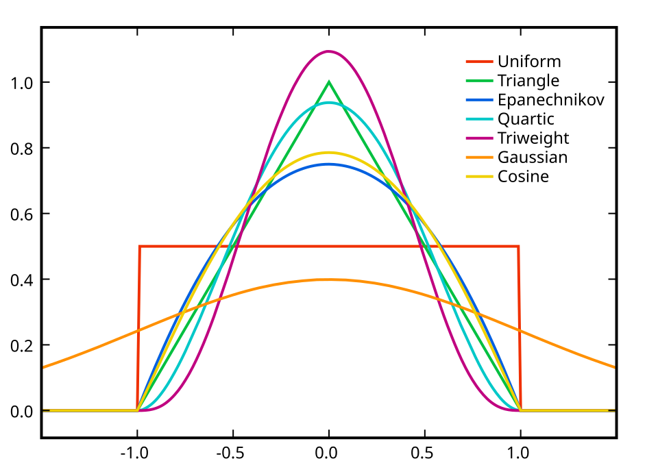
Kernel Selection

There are several types of kernels to select from. The most common selection is the Epanechnikov (parabolic) kernel. Below I provide a visualization of these kernels as well as a comparision across these kernels.

Kernel	Support	\(K(u)\)	Efficiency (relative to Epanechnikov)
Uniform (Rectangular)	\(\\|u\\| \leq 1\)	\(\frac{1}{2}\)	92.9%
Triangular	\(\\|u\\| \leq 1\)	\(1 - \\|u\\|\)	98.6%
Epanechnikov (Parabolic)	\(\\|u\\| \leq 1\)	\(\frac{3}{4}(1 - u^2)\)	100%
Quartic (Biweight)	\(\\|u\\| \leq 1\)	\(\frac{15}{16}(1 - u^2)^2\)	99.4%
Triweight	\(\\|u\\| \leq 1\)	\(\frac{35}{32}(1 - u^2)^3\)	98.7%
Tricube	\(\\|u\\| \leq 1\)	\(\frac{70}{81}(1 - \\|u\\|^3)^3\)	99.8%
Gaussian	All \(u\)	\(\frac{1}{\sqrt{2\pi}}e^{-\frac{1}{2}u^2}\)	95.1%
Cosine	\(\\|u\\| \leq 1\)	\(\frac{\pi}{4}\cos(\frac{\pi}{2}u)\)	99.9%
Logistic	All \(u\)	\(\frac{1}{e^u + 2 + e^{-u}}\)	88.7%
Sigmoid	All \(u\)	\(\frac{2}{\pi(e^u + e^{-u})}\)	84.3%

Optimal Bandwidth Selection

The choice of bandwidth \(h\) is critical for kernel matching, as it controls the trade-off between bias and variance. The most common optimality criterion is the Mean Integrated Squared Error (MISE):

\[ \text{MISE}(h) = E\left[\int \left(\hat{f}_h(x) - f(x)\right)^2 dx\right] \]

where \(\hat{f}_h(x)\) is the kernel density estimate and \(f(x)\) is the true (unknown) density function.

Under mild assumptions, the MISE can be approximated by the Asymptotic MISE (AMISE):

\[ \text{AMISE}(h) = \frac{R(K)}{nh} + \frac{1}{4}m_2(K)^2 h^4 R(f'') \]

where:

\(R(g) = \int g(x)^2 dx\) for a function \(g\)
\(m_2(K) = \int x^2 K(x) dx\) is the second moment of the kernel
\(R(f'')\) involves the second derivative of the true density
\(n\) is the sample size

The optimal bandwidth that minimizes AMISE is:

\[ h_{\text{AMISE}} = \left[\frac{R(K)}{m_2(K)^2 R(f'')}\right]^{1/5} n^{-1/5} \]

Silverman’s Rule of Thumb:

Since \(R(f'')\) is unknown in practice, the Rule of Thumb estimator provides a practical solution by assuming the underlying density is approximately normal:

\[ h_{\text{ROT}} = \left(\frac{4\hat{\sigma}^5}{3n}\right)^{1/5} \approx 1.06\hat{\sigma}n^{-1/5} \]

where \(\hat{\sigma}\) is the sample standard deviation. A more robust version uses:

\[ h_{\text{ROT}} = 0.9 \cdot \min\left(\hat{\sigma}, \frac{\text{IQR}}{1.34}\right) \cdot n^{-1/5} \]

where IQR is the interquartile range. This modification improves performance for skewed or heavy-tailed distributions. The Rule of Thumb is the default bandwidth selector in most statistical packages due to its simplicity and reasonable performance, though it may oversmooth bimodal or multimodal distributions.

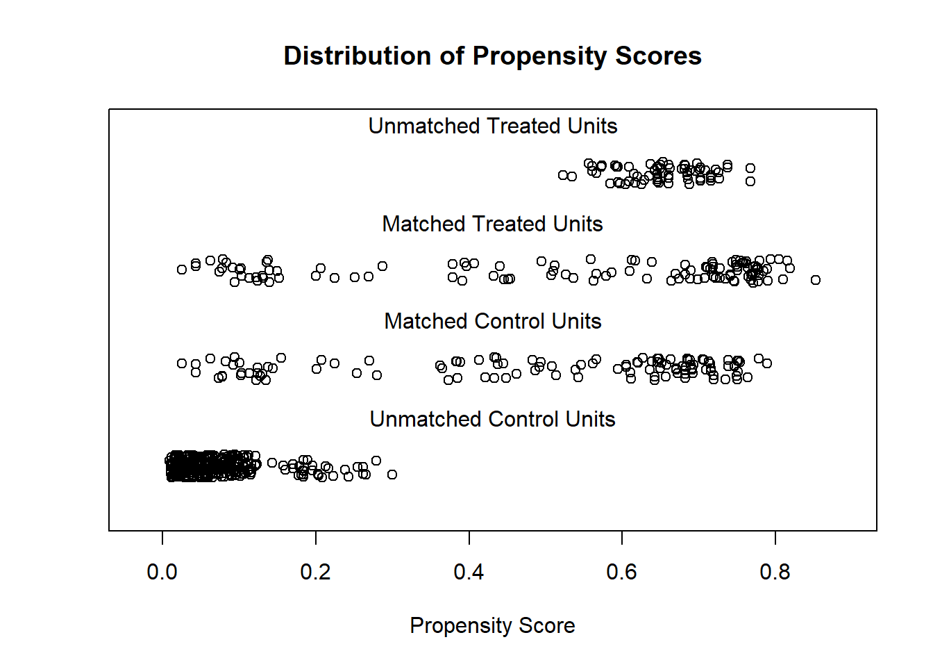
Estimation

As an example, we will explore the lalonde data set that comes with the MatchIt R package. This is data from the National Supported Work Demonstration used by Dehejia and Wahba (1999). The outcome of interest is 1978 real wages re78.

“We use data from Lalonde’s evaluation of nonexperimental methods that combine the treated units from a randomized evaluation of the NSW with nonexperimental comparison units drawn from survey datasets.”

The variables in this data are:

treat: The treatment assignment indicator is the first variable of the data frame: treatment (1 = treated; 0 = control).
age, measured in years;
education, measured in years;
black, indicating race (1 if black, 0 otherwise);
hispanic, indicating race (1 if Hispanic, 0 otherwise);
married, indicating marital status (1 if married, 0 otherwise);
nodegree, indicating high school diploma (1 if no degree, 0 otherwise);
re74, real earnings in 1974;
re75, real earnings in 1975.

# Key Matching Package
library(MatchIt, quietly = TRUE)

# Download the lalonde data 
df <- MatchIt::lalonde

# Estimate propensity scores and match
m.out <- matchit(
    treat ~ age + educ + race + married + nodegree + re74 + re75,
    data = df,
    method = "nearest",# Nearest neighbor matching
    distance = "glm",  # logistic regression
    ratio = 1,         # 1:1 matching
    caliper = 0.25,    # caliper in standard deviations
    replace = FALSE
)

# Check balance
summary(m.out, un = FALSE)


Call:
matchit(formula = treat ~ age + educ + race + married + nodegree + 
    re74 + re75, data = df, method = "nearest", distance = "glm", 
    replace = FALSE, caliper = 0.25, ratio = 1)

Summary of Balance for Matched Data:
           Means Treated Means Control Std. Mean Diff. Var. Ratio eCDF Mean
distance          0.5321        0.4892          0.1948     1.2188    0.0470
age              26.8879       26.3017          0.0819     0.4566    0.0871
educ             10.5517       10.5000          0.0257     0.6006    0.0281
raceblack         0.7500        0.7328          0.0474          .    0.0172
racehispan        0.0948        0.1034         -0.0365          .    0.0086
racewhite         0.1552        0.1638         -0.0291          .    0.0086
married           0.1983        0.2759         -0.1981          .    0.0776
nodegree          0.7155        0.6121          0.2275          .    0.1034
re74           2710.0046     2768.0725         -0.0119     1.5371    0.0512
re75           1944.4850     1931.8969          0.0039     1.6501    0.0422
           eCDF Max Std. Pair Dist.
distance     0.2672          0.1956
age          0.2672          1.4579
educ         0.1034          1.1148
raceblack    0.0172          0.0948
racehispan   0.0086          0.4739
racewhite    0.0086          0.3200
married      0.0776          0.6823
nodegree     0.1034          0.8343
re74         0.2672          0.7508
re75         0.1552          0.8402

Sample Sizes:
          Control Treated
All           429     185
Matched       116     116
Unmatched     313      69
Discarded       0       0

# Visualize overlap
plot(m.out, type = "jitter", interactive = FALSE)

# Extract matched data
matched_data <- match.data(m.out)

# Estimate treatment effect
library(lmtest, quietly = TRUE)
library(sandwich, quietly = TRUE)

fit <- lm(re78 ~ treat + age + educ + race + married + nodegree + re74 + re75,
        data = matched_data, # Data already has matches
        weights = weights # Re-weights for PSM
        )

# Robust standard errors
coeftest(fit, vcov = vcovCL, cluster = ~subclass)


t test of coefficients:

               Estimate  Std. Error t value Pr(>|t|)  
(Intercept) -2.3293e+03  3.8256e+03 -0.6089  0.54323  
treat        1.8873e+03  9.0485e+02  2.0857  0.03815 *
age         -2.5187e+00  5.0885e+01 -0.0495  0.96057  
educ         5.3057e+02  2.4030e+02  2.2079  0.02827 *
racehispan  -3.7369e+02  1.5291e+03 -0.2444  0.80716  
racewhite    6.1285e+02  1.1210e+03  0.5467  0.58515  
married      5.9076e+02  1.2424e+03  0.4755  0.63489  
nodegree     1.6133e+03  1.3913e+03  1.1595  0.24748  
re74         8.0925e-02  1.9583e-01  0.4132  0.67983  
re75         1.4340e-01  1.9686e-01  0.7284  0.46711  
---
Signif. codes:  0 '***' 0.001 '**' 0.01 '*' 0.05 '.' 0.1 ' ' 1

from causalinference import CausalModel
import pandas as pd

# Load data
data = pd.read_csv('lalonde.csv')

# Prepare data
Y = data['re78'].values
D = data['treat'].values  
X = data[['age', 'educ', 'race', 'married','nodegree', 're74', 're75']].values

# Fit model
causal = CausalModel(Y, D, X)

# Estimate propensity scores
causal.est_propensity_s()

# Match with caliper
causal.est_via_matching(matches = 1, bias_adj = True)

# Results
print(causal.estimates)

* Load data 
import delimited "lalonde.csv", clear

egen race1 = group(race)

* Estimate propensity score
logit treat age educ race1 married nodegree re74 re75

* Predict propensity scores
predict pscore, pr

* Nearest neighbor matching with caliper
psmatch2 treat, pscore(pscore) outcome(re78) caliper(0.25) ate

* Check balance
pstest age educ1 race married nodegree re74 re75, ///
    treated(treat) pscore(pscore)

Critiques of PSM

Despite its intuitive appeal, King and Nielsen (2019) show that propensity score matching often fails to achieve adequate covariate balance and can even increase imbalance compared to simpler methods.

Key Problems:

Paradox of PSM: Equal propensity scores do not guarantee similar covariates

\[ e(X_i) = e(X_j) \not\Rightarrow X_i = X_j \]

But: \[ X_i = X_j \Rightarrow e(X_i) = e(X_j) \]

Model dependence: Small changes in propensity score specification can dramatically change matches
Inefficiency: Discarding unmatched units reduces sample size unnecessarily
Approximation stochasticity: The quality of matches varies randomly based on the specific sample

Potential Better Alternatives

Covariate matching (Mahalanobis distance, CEM)
Inverse probability weighting (IPW)
Doubly robust estimators
Entropy balancing

Common Pitfalls

Including post-treatment variables in propensity score model
Ignoring lack of common support
Using p-values to assess balance (conflates sample size with balance)
Not checking covariate balance after matching
Treating estimated propensity scores as known

Recommended Workflow

Specify covariates based on domain knowledge (include all confounders)
Estimate propensity scores
Check overlap (common support)
Perform matching
Assess balance (standardized mean differences, variance ratios)
If imbalance remains: refine model or try different matching method
Estimate treatment effect on matched sample
Sensitivity analysis for potential hidden bias

References

Dehejia, Rajeev, and Sadek Wahba. 1999. “Causal Effects in Nonexperimental Studies: Reevaluating the Evaluation of Training Programs.” Journal of the American Statistical Association 94: 1053–62.

King, Gary, and Richard Nielsen. 2019. “Why Propensity Scores Should Not Be Used for Matching.” Political Analysis 27 (4): 435–54. https://doi.org/10.1017/pan.2019.11.

Rosenbaum, Paul R., and Donald B. Rubin. 1983. “The Central Role of the Propensity Score in Observational Studies for Causal Effects.” Biometrika 70 (1): 41–55. https://doi.org/10.1093/biomet/70.1.41.