Entropy balancing is a preprocessing method that reweights control observations to achieve exact covariate balance on specified moments (means, variances, skewness) while staying as close as possible to uniform weights (Hainmueller 2012).
Unlike propensity score weighting, which estimates weights indirectly through a propensity score model, entropy balancing directly solves for weights that satisfy user-specified balance constraints. This approach:
Achieves exact balance on specified moments by construction
Requires no iterative model specification searching for balance
Produces stable weights through maximum entropy optimization
Combines advantages of matching and weighting methods
The Core Insight
Traditional matching methods involve two steps:
Estimate propensity scores (or distances)
Check if resulting matches achieve balance
Entropy balancing reverses this logic:
Specify desired balance constraints directly
Solve for weights that satisfy those constraints
This guarantees balance on chosen moments without iterative model tweaking.
Mathematical Formulation
The Optimization Problem
Entropy balancing finds weights \(w_i\) for control observations (\(T_i = 0\)) that minimize:
\[
H(w) = \sum_{i: T_i=0} h(w_i)
\]
subject to balance and normalization constraints.
Objective Function
The objective uses a distance metric (typically Shannon entropy):
\[
h(w_i) = w_i \log(w_i / q_i)
\]
where \(q_i\) is a base weight (typically \(q_i = 1\) for uniform base weights).
This is equivalent to minimizing the Kullback-Leibler divergence from the base weights, ensuring weights are as uniform as possible while satisfying constraints.
Balance Constraints
The key constraints enforce exact balance on covariate moments:
Moment balance constraints:\[
\sum_{i: T_i=0} w_i c_{ri}(\mathbf{X}_i) = \sum_{j: T_j=1} c_{rj}(\mathbf{X}_j) \quad \text{for } r = 1, \ldots, R
\]
where \(c_r(\mathbf{X})\) are covariate moment functions.
Normalization Constraint
Weights must sum to the number of controls:
\[
\sum_{i: T_i=0} w_i = N_0
\]
where \(N_0\) is the number of control observations.
Balance Measures
              Type Diff.Adj
age        Contin.       -0
educ       Contin.       -0
racehispan  Binary        0
racewhite   Binary       -0
married     Binary       -0
nodegree    Binary        0
re74       Contin.       -0
re75       Contin.       -0

Effective sample sizes
           Control Treated
Unadjusted  429.       185
Adjusted     98.46     185
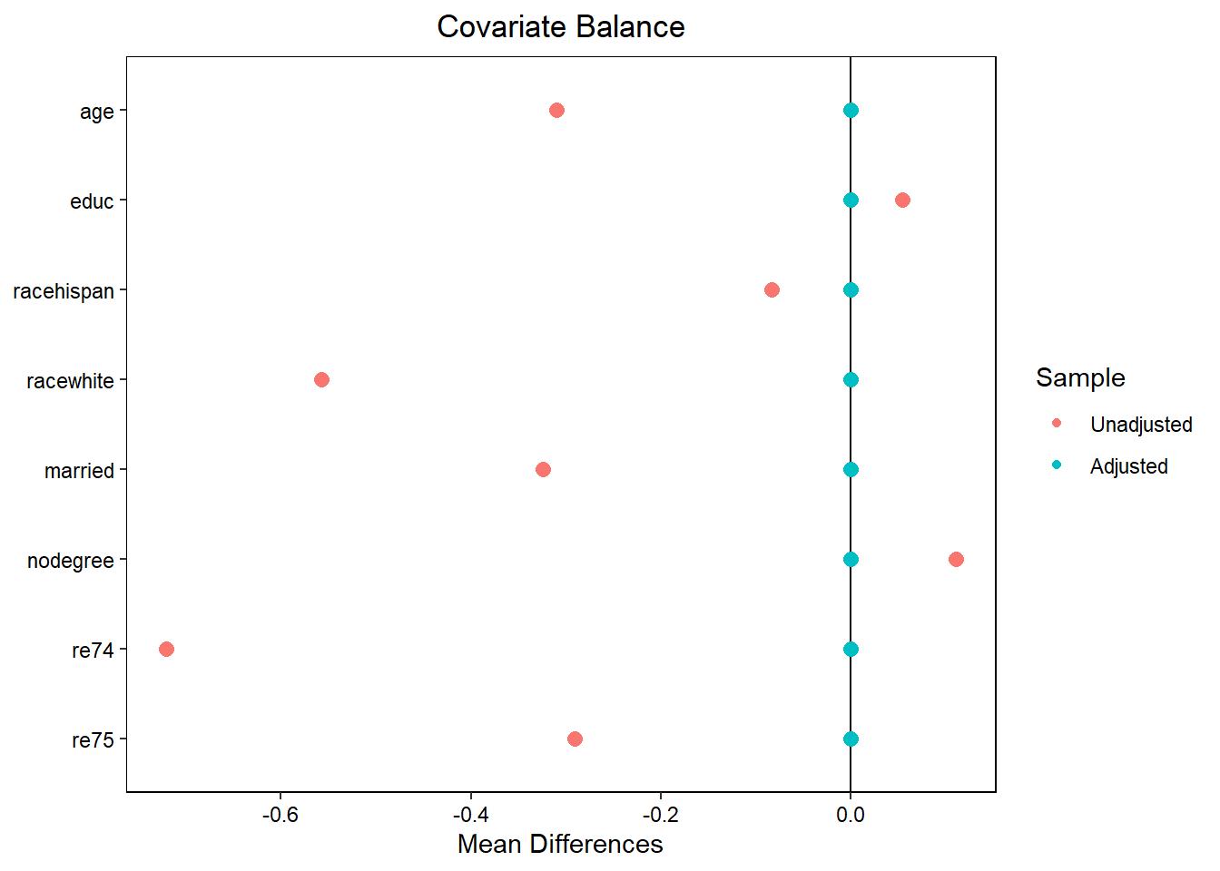
love.plot(eb_fit, treat = T_vec, covs = X) # Love plot of standardized mean differences
Warning: Standardized mean differences and raw mean differences are present in the same
plot. Use the `stars` argument to distinguish between them and appropriately
label the x-axis. See `love.plot()` for details.
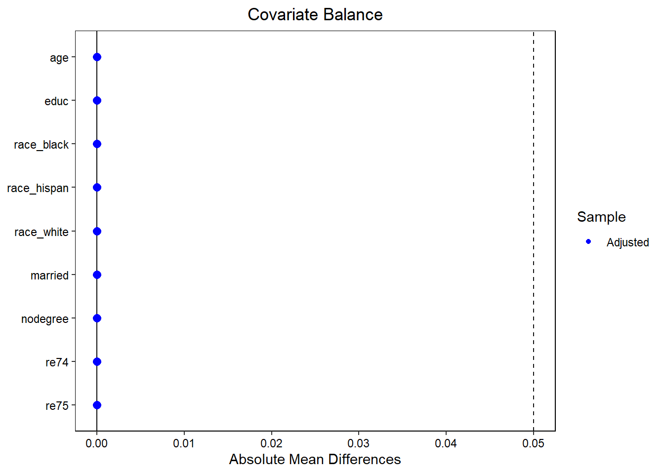
# Extract weightsdata$weight <-1# Initialize all weights to 1data$weight[data$treat ==0] <- eb_fit$w# Verify balancebal_check <-bal.tab( treat ~ age + educ + race + married + nodegree + re74 + re75,data = data,weights ="weight",method ="weighting",stats =c("m", "v"),thresholds =c(m =0.05, v =2))print(bal_check)
Balance Measures
               Type Diff.Adj     M.Threshold V.Ratio.Adj      V.Threshold
age         Contin.       -0 Balanced, <0.05      0.4096 Not Balanced, >2
educ        Contin.       -0 Balanced, <0.05      0.6635     Balanced, <2
race_black   Binary        0 Balanced, <0.05           .
race_hispan  Binary        0 Balanced, <0.05           .
race_white   Binary       -0 Balanced, <0.05           .
married      Binary       -0 Balanced, <0.05           .
nodegree     Binary        0 Balanced, <0.05           .
re74        Contin.       -0 Balanced, <0.05      1.3265     Balanced, <2
re75        Contin.       -0 Balanced, <0.05      1.3351     Balanced, <2

Balance tally for mean differences
                    count
Balanced, <0.05         9
Not Balanced, >0.05     0

Variable with the greatest mean difference
 Variable Diff.Adj     M.Threshold
     re74       -0 Balanced, <0.05

Balance tally for variance ratios
                 count
Balanced, <2         3
Not Balanced, >2     1

Variable with the greatest variance ratio
 Variable V.Ratio.Adj      V.Threshold
      age      0.4096 Not Balanced, >2

Effective sample sizes
           Control Treated
Unadjusted  429.       185
Adjusted     98.46     185
Warning: Unadjusted values are missing. This can occur when `un = FALSE` and `quick =
TRUE` in the original call to `bal.tab()`.
Warning: `var.order` was set to "unadjusted", but no unadjusted mean differences were
calculated. Ignoring `var.order`.
Warning: Standardized mean differences and raw mean differences are present in the same
plot. Use the `stars` argument to distinguish between them and appropriately
label the x-axis. See `love.plot()` for details.
Trim sample: Remove units with extreme covariate values
Relax constraints: Balance fewer moments
Use covariate adjustment: Include covariates in outcome model
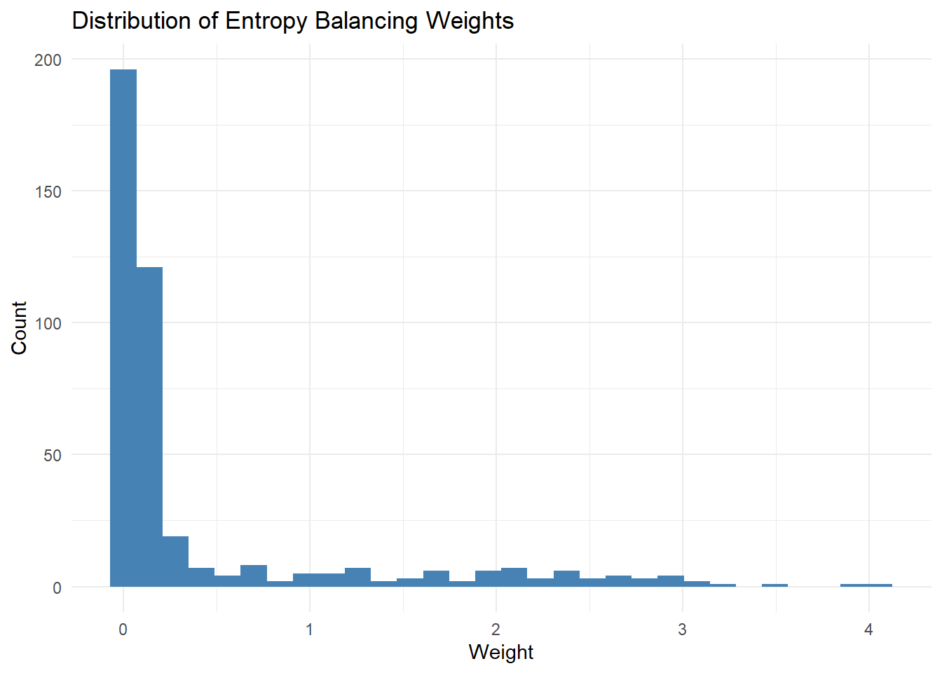
# Check for extreme weightsquantile(eb_weight, c(0.95, 0.99, 1.0))# Flag extreme weightsextreme <- eb_weight >quantile(eb_weight, 0.99)table(extreme)
Diagnostics
Balance Checks
# Standardized mean differences should be ~0bal.tab(treat ~ age + educ + race + married + nodegree + re74 + re75, data = df,weights ="weight",stats ="m")# Variance ratios should be ~1bal.tab(treat ~ age + educ + race + married + nodegree + re74 + re75,data = df, weights ="weight",stats ="v")
# Create interaction termsdf$age_edu <- df$age * df$education# Include in balancingebalance(treatment, X =cbind(age, education, age_edu))
Stable Balancing Weights
Extension by Zhao and Percival (2017) adds stability constraints:
\[
\min H(w) \quad \text{s.t. balance and } \max(w_i) \leq M
\]
Kernel Balancing
Hazlett (2020) proposes kernel-based approach for nonlinear balance.
References
Key papers on entropy balancing:
Hainmueller (2012) - Original entropy balancing method
Zhao and Percival (2017) - Stable balancing weights extensions
Hazlett (2020) - Kernel balancing for nonparametric balance
Vegetabile et al. (2021) - Nonparametric preprocessing methods
References
Hainmueller, Jens. 2012. “Entropy Balancing for Causal Effects: A Multivariate Reweighting Method to Produce Balanced Samples in Observational Studies.”Political Analysis 20 (1): 25–46. https://doi.org/10.1093/pan/mpr025.
Hazlett, Chad. 2020. “Kernel Balancing: A Flexible Non-Parametric Weighting Procedure for Estimating Causal Effects.”Statistica Sinica 30 (3): 1155–89. https://doi.org/10.5705/ss.202018.0122.
Vegetabile, Brian G., Beth Ann Griffin, Donna L. Coffman, Matthew Cefalu, Michael W. Robbins, and Daniel F. McCaffrey. 2021. “Nonparametric Estimation of Population Average Dose-Response Curves Using Entropy Balancing Weights for Continuous Exposures.”Health Services and Outcomes Research Methodology 21 (1): 69–110. https://doi.org/10.1007/s10742-020-00236-2.
Zhao, Qingyuan, and Daniel Percival. 2017. “Entropy Balancing Is Doubly Robust.”Journal of Causal Inference 5 (1). https://doi.org/10.1515/jci-2016-0010.