When the number of candidate covariates is large, standard propensity score modeling can overfit and produce unstable matches. A common strategy is to estimate the propensity score with LASSO-regularized logistic regression, which performs shrinkage and variable selection simultaneously (Tibshirani 1996).
In this context, “LASSO matching” means:
Estimate treatment propensity with penalized logistic regression.
Use the resulting propensity scores for matching (nearest neighbor, caliper, or subclassification).
Check balance and estimate treatment effects on the matched sample.
LASSO Refresher
LASSO (Least Absolute Shrinkage and Selection Operator) solves
Call:
matchit(formula = treat ~ 1, data = df, method = "nearest", distance = df$ps_lasso,
replace = FALSE, caliper = 0.2, std.caliper = TRUE)
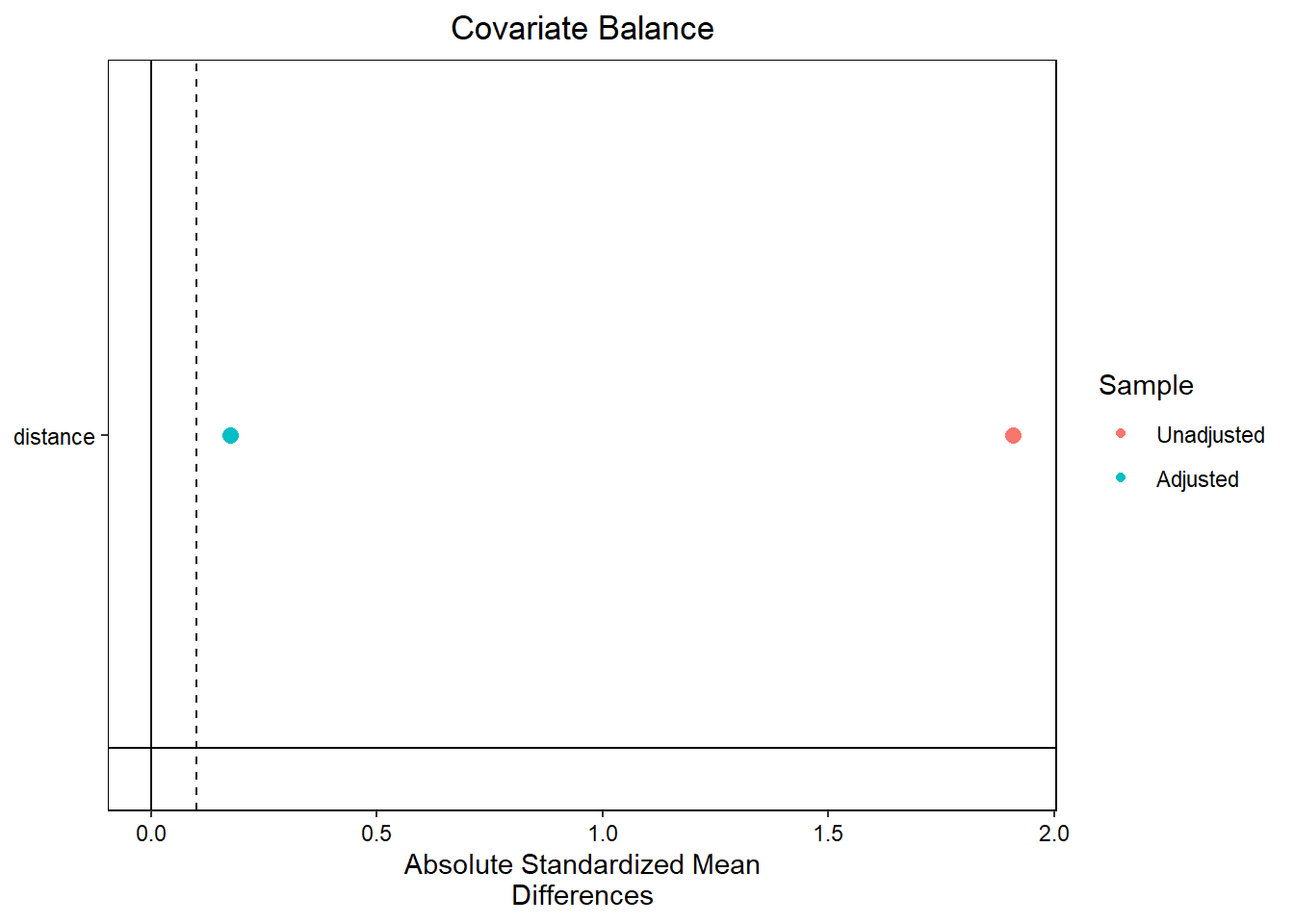
Summary of Balance for All Data:
Means Treated Means Control Std. Mean Diff. Var. Ratio eCDF Mean
distance 0.5855 0.1787 1.9085 0.9842 0.3965
eCDF Max
distance 0.6676
Summary of Balance for Matched Data:
Means Treated Means Control Std. Mean Diff. Var. Ratio eCDF Mean
distance 0.5148 0.4778 0.1738 1.1906 0.037
eCDF Max Std. Pair Dist.
distance 0.2252 0.1741
Sample Sizes:
Control Treated
All 429 185
Matched 111 111
Unmatched 318 74
Discarded 0 0
Call:
lm(formula = re78 ~ treat, data = matched, weights = weights)

Residuals:
   Min     1Q Median     3Q    Max
 -7095  -5094  -2792   3044  53213

Coefficients:
            Estimate Std. Error t value Pr(>|t|)
(Intercept)   5094.3      708.8   7.188 1.01e-11 ***
treat         2000.8     1002.4   1.996   0.0472 *
---
Signif. codes:  0 '***' 0.001 '**' 0.01 '*' 0.05 '.' 0.1 ' ' 1

Residual standard error: 7467 on 220 degrees of freedom
Multiple R-squared:  0.01779,   Adjusted R-squared:  0.01332
F-statistic: 3.984 on 1 and 220 DF,  p-value: 0.04716
L1 Logistic + Matching
import numpy as npimport pandas as pdfrom sklearn.linear_model import LogisticRegressionCVfrom sklearn.preprocessing import StandardScalerfrom sklearn.pipeline import make_pipeline# Load datadata = pd.read_csv('lalonde.csv')# Suppose df has columns: treat, outcome, and covariatescovars = ["age", "educ", "married", "nodegree", "re74", "re75"]X = df[covars].to_numpy()y = df["treat"].to_numpy()# L1-penalized logistic with CVclf = make_pipeline( StandardScaler(), LogisticRegressionCV( penalty="l1", solver="saga", cv=10, scoring="neg_log_loss", max_iter=5000, n_jobs=-1, refit=True ))clf.fit(X, y)ps = clf.predict_proba(X)[:, 1]df["ps_lasso"] = np.clip(ps, 1e-6, 1-1e-6)# Then perform nearest-neighbor matching on ps_lasso# (using your preferred matching package/tool)
Penalized PS then Match
* Load dataimport delimited "lalonde.csv", clear* 1) Fit lasso-logit propensity modellasso logit treat age educ i.race married nodegree re74 re75* 2) Predict propensity scorespredictdouble ps_lasso, pr* 3) Match using propensity score* (psmatch2 is user-written)psmatch2 treat, pscore(ps_lasso) outcome(re78) neighbor(1) caliper(0.2)* 4) Check balancepstest age educ married nodegree re74 re75, both
Practical Considerations
Tuning Parameter Choice
lambda.min: better in-sample fit, less sparse.
lambda.1se: more stable and parsimonious (often preferred for design stages).
Include Interactions Thoughtfully
High-dimensional sets can include interactions and nonlinear terms, but retain only pre-treatment features.
Do Not Skip Diagnostics
A good propensity model is one that yields balance, not just high Area Under the Receiver Operating Characteristic Curve (AUC-ROC).
Connection to High-Dimensional Treatment Effect Literature
The high-dimensional treatment-effect literature emphasizes that regularization can reduce overfitting and improve precision, but valid inference still requires careful design and diagnostics. Bloniarz et al. show that LASSO-based adjustment can improve efficiency and recommend a practical two-step variant (LASSO selection followed by OLS refit) in some settings (Bloniarz et al. 2016).
For observational matching, this translates to a pragmatic approach:
Use LASSO to stabilize propensity estimation and feature selection.
Match on the estimated score.
Validate balance rigorously.
Report sensitivity analyses.
Reporting Checklist
Candidate covariate set and feature engineering.
LASSO specification (family, alpha, CV folds).
Tuning rule (lambda.min or lambda.1se).
Matching algorithm and caliper choice.
Balance diagnostics before and after matching.
Effective sample size and discarded units.
Outcome model and uncertainty method.
References
Bloniarz, Adam, Hanzhong Liu, Cun-Hui Zhang, Jasjeet S. Sekhon, and Bin Yu. 2016. “Lasso Adjustments of Treatment Effect Estimates in Randomized Experiments.”Proceedings of the National Academy of Sciences of the United States of America 113 (27): 7383–90. https://doi.org/10.1073/pnas.1510506113.
Tibshirani, Robert. 1996. “Regression Shrinkage and Selection via the Lasso.”Journal of the Royal Statistical Society: Series B (Methodological) 58 (1): 267–88. https://doi.org/10.1111/j.2517-6161.1996.tb02080.x.